Model architecture labels can make a model page feel more complicated than it needs to be. You do not need to understand every internal detail to choose a model. You only need to know how these labels affect memory use, speed, and the way you compare models.
Dense Models
Most models you will encounter are dense models. When a dense model processes a token, it uses all of its parameters for that calculation. This is how all the frontier models you are used to work.
A 7B dense model has roughly 7 billion parameters, and each generated token uses the whole model. This makes the parameter count a useful starting point for estimating how much memory the model needs and how fast it might run.
Dense models are straightforward to compare, but parameter count is still not a quality score. A newer 7B model can outperform an older or differently trained 13B model on a specific task.
Since dense models require all of their parameters to be used for every token, they tend to be the slowest option and the most memory intensive, but they often produce better results.
Mixture Of Experts
A mixture-of-experts, or MoE, model has multiple expert networks inside some of its layers. Each expert is essentially a smaller neural network that works very similar to the full model.
The model also has a router. For every token, the router decides which few experts should process that token. This is where the name mixture of experts comes from.
Imagine you ask a model to create a React component and write a Python test for it. One expert may have learned patterns that are especially useful for frontend JavaScript, while another may be better at Python. The router can activate both of those experts while leaving unrelated experts inactive.
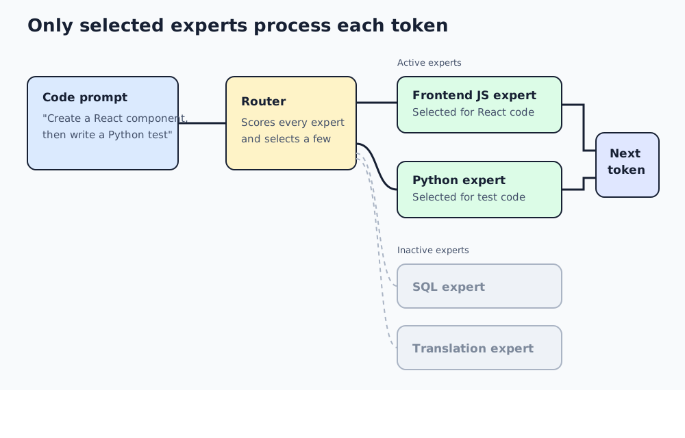
This example is abstract. Experts are not labeled frontend or Python inside a real model, and one expert can help with many kinds of patterns. The useful mental model is that the router learns which experts are most useful for the current token.
You may see an MoE model named like this:
8x7B
or
A3B
In the first example this says the model has 8 experts that are each 7B parameters large. The second example doesn't say how many experts the model has but is says that there are only ever 3B parameters active for each token generation.
MoE Benefits
MoE models have a few specific benefits compared to dense models.
Speed
MoE models are significantly faster than dense models of the same total parameter count since MoE models only use a small portion of the total parameters on each token generation.
CPU Offload
This is a bit of an advanced benefit, but if you entire model does not fit into the VRAM of your GPU, you can offload just some layers of the MoE model to the CPU. This will drastically reduce your speed, but it allows you to run larger models than your GPU alone could handle.
This essentially works by loading all the important parts of the model on the GPU while offloading the less frequently used layers to the CPU.
Demo
Let me show you an example of how this CPU offload can allow me to load a model my GPU normally couldn't run at all.
Without using MoE offload I get 1-3 tokens per second, but with MoE I can manage 50 tokens per second.
MoE Tradeoffs
The only major downside to MoE models is that they tend to produce lower quality outputs compared to a dense model of the same total parameter count. The only reason to use MoE over a dense model is if you need the speed increase or you have hardware constraints that prevent you from running a dense model of the same size.
The reduction in quality is overall pretty minimal, but can be noticeable in certain complex tasks.
Try MoE Yourself
Now I want you to try out an MoE model yourself. The LFM2.5-8B-A1B model you downloaded earlier happens to be an MoE model, so you can experiment with it to see the benefits and tradeoffs discussed above. Compare the speed to the Qwen 2.5 Coder 0.5B model we downloaded earlier. (You can also compare to Qwen3.5-9B to see how it performs against a dense model of similar size).
You should notice that even though the LFM model is about 16x larger it runs at comparable speeds to the Qwen model since it only activates a small portion of its total parameters for each token generation.
Also, try experimenting with offloading some layers to the CPU and observe how it affects the speed and memory usage of the model (this is really only useful if you do not have unified memory).
Multi-Token Prediction
Most language models predict one token at a time. Multi-token prediction, or MTP, is an architecture feature that lets a model predict more than one future token during a generation step.
The goal is to improve generation speed. A model that can accurately predict multiple upcoming tokens may need fewer full passes through the model to produce the same response which can result in 1.5x-2x increases in speed.
MTP models may not always increase speed, though, so I recommend testing it with your specific prompts and hardware to see if it provides a benefit. Also, MTP models take up more memory since they need to store multiple predicted tokens at once which can be a limiting factor on devices with less memory.
Try MTP Yourself
First I will show you how MTP affects the generation speed for me and then you can try it yourself.
Use the Qwen3.5-9B model we downloaded earlier for this experiment. Start by enabling MTP with the default settings and note the speed. Next disable MTP and note the new speed. You may need to use larger or more complex prompts to see a true difference. You can use the prompt Write a JavaScript class for a linked list if you want.
You can even try playing with the MTP settings to make it generate more or less tokens at once.